Improve your Scientific Models with Meta-Learning and Likelihood-Free Inference

23 Dec 2018 on Machine Learning

Note: This post was first published as a Medium Article for Towards Data Science

Introduction to likelihood-free inference and distillation of the paper Recurrent Machines for Likelihood-Free Inference, published at the NeurIPS 2018 Workshop on Meta-Learning.

Article jointly written by Arthur Pesah and Antoine Wehenkel

Motivation

There are usually two ways of coming up with a new scientific theory:

• Starting from first principles, deducing the consequent laws, and coming up with experimental predictions in order to verify the theory
• Starting from experiments and inferring the simplest laws that explain your data.

The role of statistics and machine learning in science is usually related to the second kind of inference, also called induction.

Imagine for instance that you want to model the evolution of two populations (let’s say foxes and rabbits) in an environment. A simple model is the Lotka-Volterra differential equation: you consider the probability that an event such as “a fox eating a rabbit”, “a rabbit being born”, “a fox being born”, etc. happens in a small time interval, deduce a set of differential equations depending on those probabilities, and predict the evolution of the two animals by solving those equations. By comparing your prediction with the evolution of a real population, you can infer the best model parameters (probabilities) in this environment.

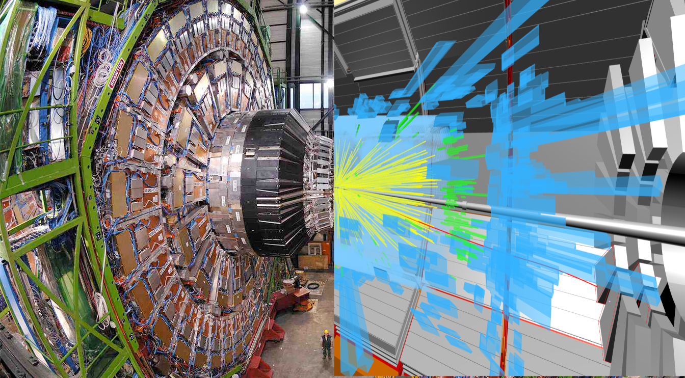
Modern theories require simulations in order to be linked to observations. It can be either a simple differential equation solver as in the case of the Lotka-Volterra model, or a complex Monte-Carlo simulator as they use in particle physics for instance.

By comparing the results of a simulation, i.e. the predictions of a model, with real data, it is then possible to know the correctness of your model and adjust it accordingly. If this process of going back and forth between the model and the experimental data is usually done manually, the question that any machine learning practitioner would ask is: can we do it automatically? Can we build a machine that takes a tweakable simulator and real data as input, and returns the version of the simulator that fits best some real data?

That’s the object of our recent work¹, where we trained a neural network to come up with the best sequence of simulator tweaks in order to approximate experimental data, capitalizing on the recent advances in the fields of likelihood-free inference and meta-learning.

Likelihood-free inference

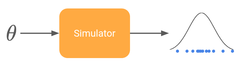
Let’s rephrase our problem in a more formal way. We can model a simulator (also called generative model) by a stochastic function that takes some parameters $\theta$ and returns samples $x$ drawn from a certain distribution (the so-called model).

This formalism applies to any scientific theory that includes randomness, as it’s very often the case in modern science (particle collisions are governed by the law of quantum physics which are intrinsically random, biological processes or chemical reactions often occur in a noisy environment, etc.).

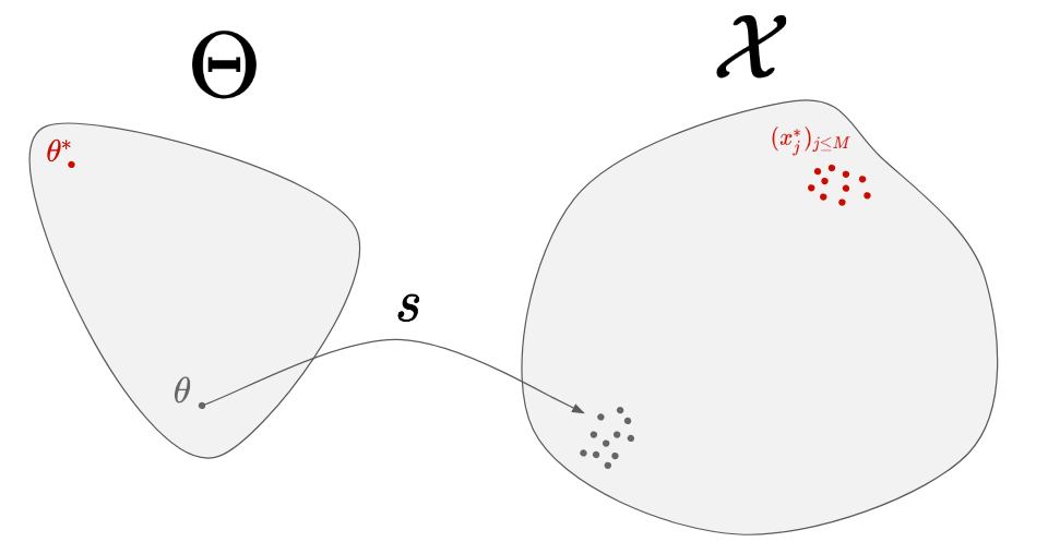
Experimental data consist in a set of points living in the same space as the output of the simulator. The goal of inference is then to find the parameters $\theta$ such that the simulator generate points as close as possible to the real data.

Scientific fields using such simulators include:

• Population genetics. Model: Coalescent theory. Observation: the DNA of a current population. Parameters: the DNA of the common ancestor.
• High-energy particle physics. Model: Standard Model of particle physics. Observation: output of the detector during a collision. Parameters: coupling constants of the Standard Model (like the mass of the particles or the strength of the different forces).
• Computational neuroscience. Model: Hodgkin-Huxley model. Observation: evolution of the voltage of a neuron after activation. Parameters: biophysical parameters of the neuron.

So how can we predict the parameters of a simulator given some real observations? Let’s consider the simple example of a Gaussian simulator, that takes a vector $\theta=(\mu,\sigma)$ as parameters and returns samples from the Gaussian distribution $\mathcal{N}(\mu,\sigma)$.

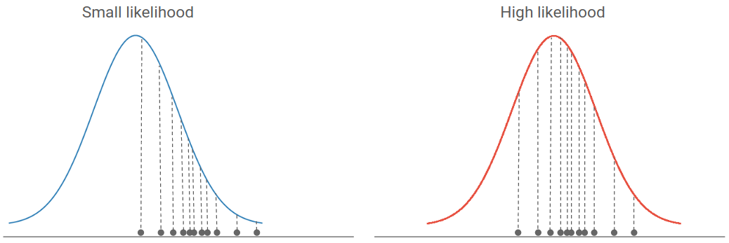
The classical way to infer the parameters of such a simulator is called Maximum Likelihood Estimation (MLE). The likelihood is defined as the density of the real data under a parametric model. It means that if most data points are located in high density regions, the likelihood will be high. Hence, the best parameters of a model are often the ones that maximize the likelihood of real data. If you are unfamiliar with likelihood-based inference, you can read this excellent introduction to the subject.

If you have explicitly access to the underlying probability distribution of your simulator, as well as the gradient of this distribution, you can for instance perform a gradient descent in the parameters space, in order to maximize the likelihood and infer the best parameters of your model.

However, many real-life simulators have an intractable likelihood, which means that the explicit probability distribution is too hard to compute (either analytically or numerically) . We must therefore find new ways to infer the optimal parameters without using neither the likelihood function nor its gradient.

To sum it up, we have a black-box stochastic simulator that takes parameters and generates samples from an unknown probability distribution, as well as real data that we are able to compare to the generated ones. Our goal is to find the parameters that lead the simulator to generate data as close as possible to the real ones. This setting is called likelihood-free inference.

How can we likelihood-free infer?

Let’s try to come up progressively with a method to solve our problem. The first thing we can do is to start from a random parameter, and simulate the corresponding data:

Representation of the two spaces of interest. The true parameter (that we wish to infer) is the red point on the left. The real data correspond to the red cloud of points on the right. We start by choosing a random parameter θ (in gray on the left) and simulating the corresponding data points (in gray on the right)

By doing so, we can see how far our generated data are from the real data, but we have no way to know where to move in the parameter-space. Instead, let’s simulate several parameters:

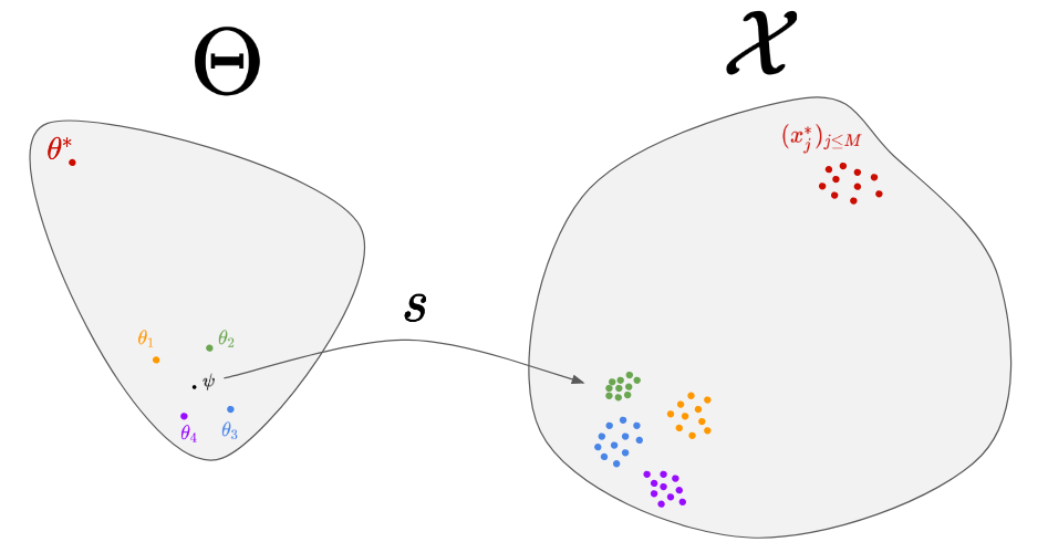
To do so, we consider a distribution in the parameter-space, called proposal distribution and noted $q(\theta|\psi)$. If we choose $q$ to be a Gaussian distribution, we will have $\psi=(\mu,\sigma)$. The first step consists in initializing $\psi$ randomly. In the figure above, we considered $\psi=\mu$ for simplicity. Then, we can perform the following step until convergence:

• Sampling a few parameters from the proposal distribution: 4 parameters around $\psi$ in the figure.
• Generating data from them: the 4 cloud of points on right.
• Choosing a good direction to move $\psi$.

The third step is the hard one. Intuitively, you would like to move $\psi$ towards the orange and green parameters, since the corresponding predictions (orange and green cloud of points) are the closest to the real data. A set of methods, called natural evolution strategies ², allow you to link the performance of each $\theta$ (in terms of similarity between its predictions and the real data) to a direction in the parameter space. A recent paper ³ use for instance the similarity measure given by a Generative Adversarial Network (GAN) to find the best direction. Even though those algorithms perform well in the general case, one can wonder if for a given simulator, it is not possible to find a better algorithm that would exploit the particular properties of this simulator. That’s where meta-learning comes into play!

Meta-learning for optimization

The idea behind meta-learning is to learn how to learn, and in our case to learn the optimization process. The main idea, introduced in the paper Learning to learn gradient descent by gradient descent⁴, is to use a recurrent neural network (RNN) to find the best descent direction at each iteration. Below is an example of sequence of points produced by a randomly initialized RNN:

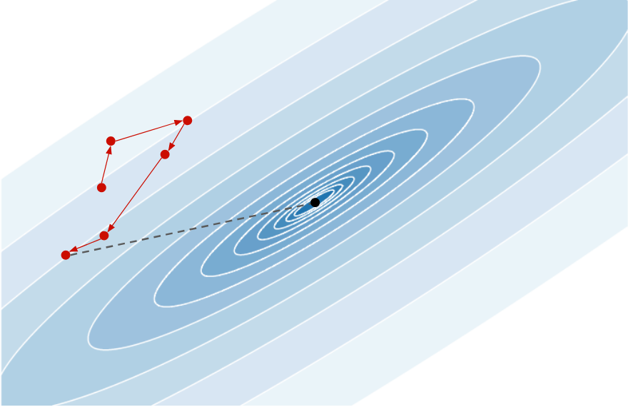
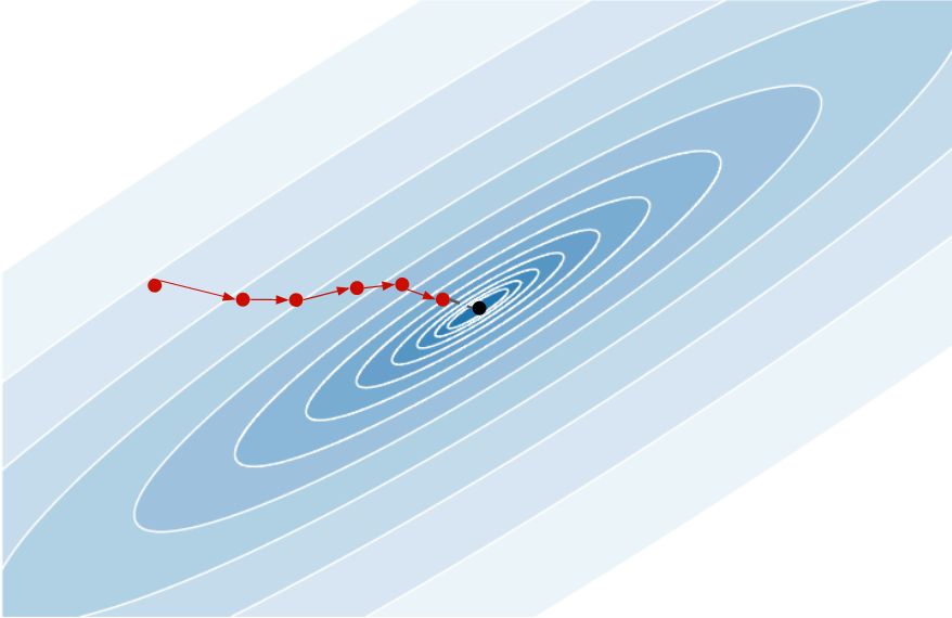
Each descent direction is random and the last point produced is far from the minimum. During training, it should learn to exploit the gradient information at each point in order to move toward the minimum, giving something like:

So how to train it? Generate many functions whose you know the minimum, and ask the RNN to minimize the distance between the last point of the sequence and the real minimum.

Learning to learn scientific models

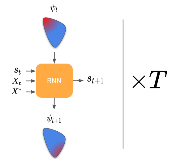
In the case of likelihood-free inference, the RNN should return a sequence of proposal parameters $\psi$, given the real observations and the generated cloud of points at each step.

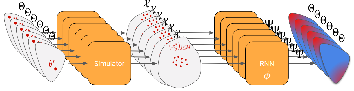
Now, same question as for learning to learn by gradient descent, how do we train the RNN? Here, the trick is to generate many random parameters θ and to pretend for each one that it is the “true parameter”. We can then simulate each θ generated and obtain a set of “real observations”. The RNN can then be trained by passing it those real observations, looking at its final proposal distribution, and comparing it to the true parameter (that we know because we have generated it).

Let’s go through an example to clarify all of that. In the figures below, the proposal distribution is represented in color (red = high density). At the beginning, the RNN is initialized randomly and we evaluate it on our first generated true parameter $\theta$ (in red).

We can then backpropagate the loss into the RNN. After repeating this process for 200 different “true parameters”, this is what is should look like:

We can see that it has learnt to exploit the information of the observation space to move towards the good parameter.

Results

We evaluated our model on different toy simulators, some where we the likelihood is known and some where it is not.

Non-likelihood-free problem: Poisson Simulator

Example of Poisson distributions for various parameters. Source: Wikipedia

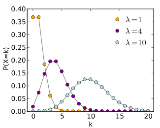
The first simulator takes a parameter λ and draw samples from a Poisson distribution $P(\lambda)$. The goal of this example was to see if we obtain comparable performance as the maximum likelihood estimator. Here are the results:

Comparison of ALFI (Automatic Likelihood-Free Inference, the name of our model), to a maximum likelihood estimator (MLE). Those box-plots represent the distribution of the mean-squared errors between the true parameters and the expected value of the final proposal distributions.

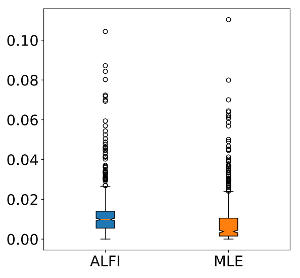
We can see that the performance are comparable, even though we didn’t give our model access to the likelihood.

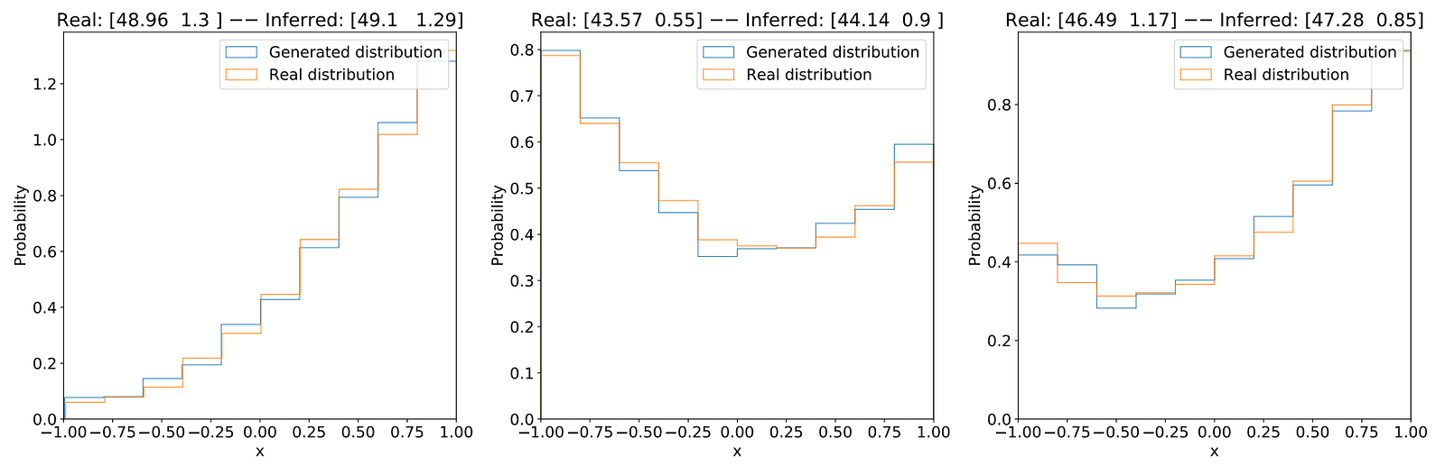
Likelihood-free problem: Particle Physics Simulator

To evaluate our model in a true likelihood-free setting, we considered a simplified particle physics model that simulate the collision of an electron and a positron turning into a muon and an antimuon.

Feynman diagram of the simulated process

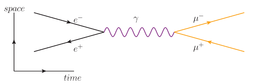
The parameters of the simulator are the energy of the incoming particles and the Fermi constant, and the output is the angle between the two muons.

To evaluate our method, we compared the real observations with the ones generated by the last parameter found. Here are the results:

Results of our method on a simple particle physics model. Comparison of our the real observations (angles of the produced particles) with the ones generated by our predicted parameter.

Discussion

We saw what likelihood-free inference is and how meta-learning can be used to solve it by learning the best sequence of simulator tweaks to fit a model to the reality.

As most meta-learning models, a limitation is that it is hard to train. We had trouble scaling our method to more complex simulators, since meta-training requires a lot of simulator calls, which might be very slow in real-world settings. However, as the field of meta-learning makes progress, we hope that new methods will emerge to alleviate this problem and make it more scalable.

1. A. Pesah, A. Wehenkel and G. Louppe, Recurrent Machines for Likelihood-Free Inference (2018), NeurIPS 2018 Workshop on Meta-Learning ↩︎

2. D. Wierstra, T. Schaul, T. Glasmachers, Y. Sun, J. Peter, J. Schmidhuber, Natural Evolution Strategies (2014), Journal of Machine Learning Research (JMLR). ↩︎

3. G. Louppe, J. Hermans, K. Cranmer, Adversarial Variational Optimization of Non-Differentiable Simulator (2017), arXiv e-prints 1707.07113 ↩︎

4. M. Andrychowicz, M. Denil, S. Gomez, M. W. Hoffman, D. Pfau, T. Schaul, B. Shillingford, N. de Freitas, Learning to learn gradient descent by gradient descent (2016), NIPS 2016 ↩︎