Introduction to Domain Adaptation
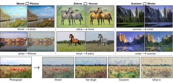
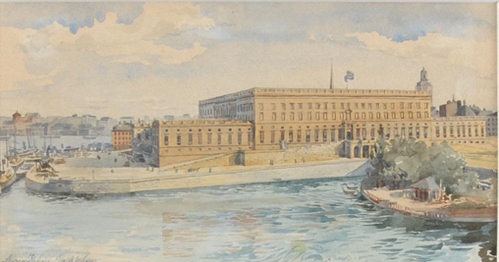
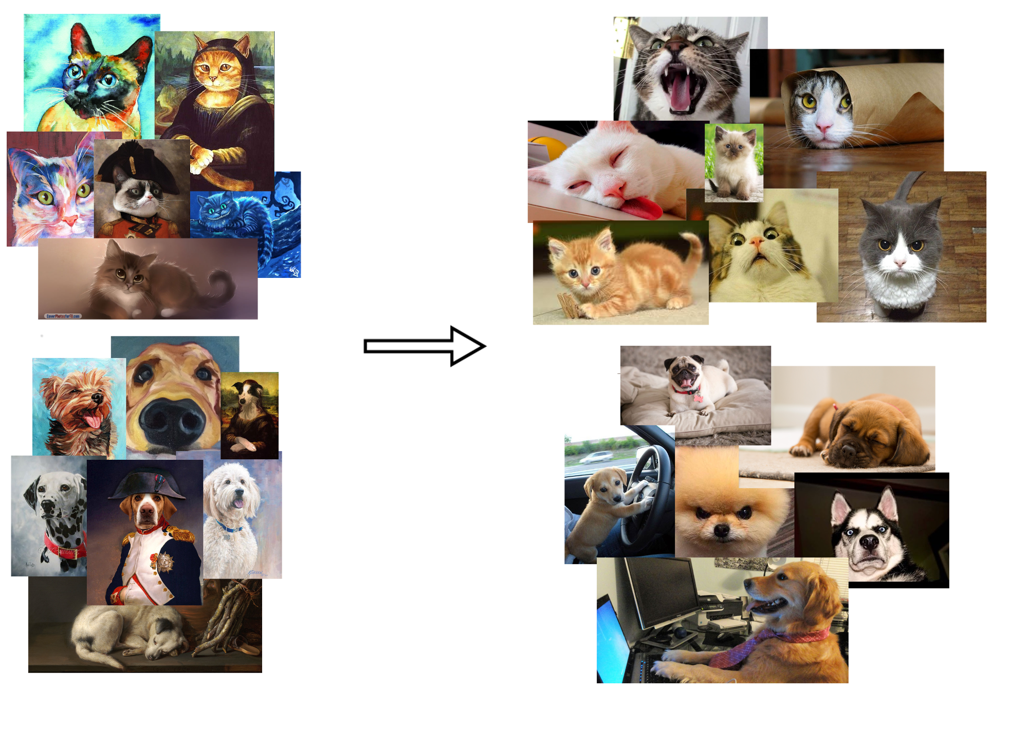
Stockholms Slott − Anna Palm de Rosa
|
Photo day 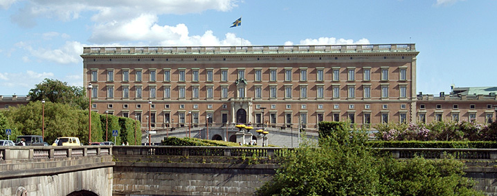
|
Photo night 
|
|
Painting black and white 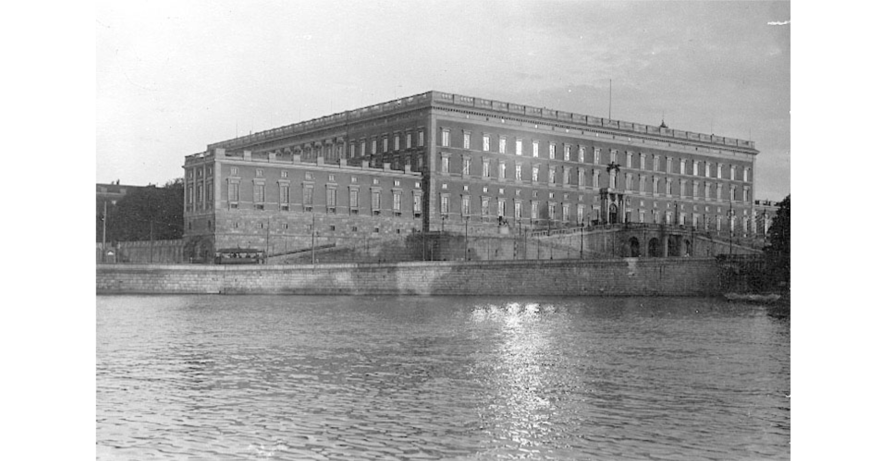
|
Painting color
|
That's what we call...
...domain adaptation
Domain adaptation
One task (classification, segmentation...)
Two datasets
|
Target − paintings Unlabeled or semi-labeled |
Source − photos Fully labelled |
Applications
|
Calibration (physics, biology...) 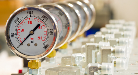
|
Simulation vs Reality 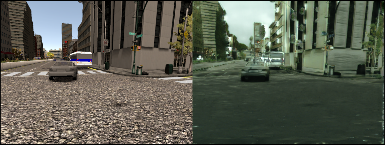
|
|
Sentiment analysis between different categories 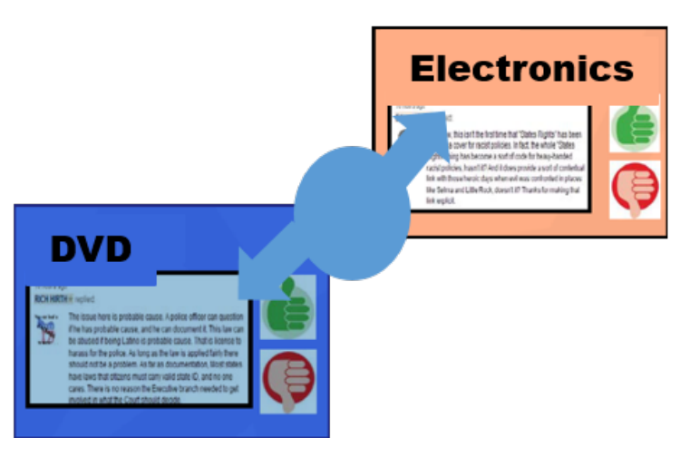
|
Adaptation between cameras 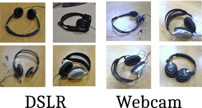
|
Relation with transfer learning
Different flavours of domain adaptation
| Source | Target | |
|---|---|---|
| Unsupervised domain adaptation | Fully labeled | Fully unlabeled |
| Semi-supervised domain adaptation | Fully labeled | Partially labeled |
| Few-shot domain adaptation | Fully labeled | Few samples |
Classical model of domain adaptation
- Probabilistic perspective: we consider two distributions $P(X_s, Y_s)$ and $P(X_t, Y_t)$ for source and target samples/labels
-
Discrepency between the domains:
\[
\epsilon_T(h) \leq \epsilon_S(h) + \frac{1}{2} d_{H\Delta H}(X_s, X_t) + \lambda(VC)
\]
where $h \in \mathcal{H}$ is a classifier, $\epsilon_{S/T}$ the error on the source/target distribution and
\[ d_{H\Delta H}(X_s, X_t) = 2 \sup_{h,h' \in \mathcal{H}} | \mathbb{E}_{x \sim X_s}[h(x) \neq h'(x)] - \mathbb{E}_{x \sim X_t}[h(x) \neq h'(x)] | \] - Goal: finding $f: \chi_s \rightarrow \chi_t$ to minimize $\frac{1}{2} d_{H \Delta H}(X_s, f(X_t))$ and $h$ to minimize $\epsilon_S(h)$
Classical model of domain adaptation
\[ d_{H\Delta H}(X_s, X_t) = 2 \sup_{h,h' \in \mathcal{H}} | \mathbb{E}_{x \sim X_s}[h(x) \neq h'(x)] - \mathbb{E}_{x \sim X_t}[h(x) \neq h'(x)] | \]
|
Hypothesis 1 |
Hypothesis 2 |
|

|
To which extent can we find two hypothesis very similar in one domain, but very different in the other
Classical model of domain adaptation
- But this theoretical distance is hard to compute, so even harder to minimize with any classicial optimization algorithm... We have to find other distances
- In probability theory, we often use divergences
- $D(P, Q) \geq 0$ for all $P,Q \in S$
- $D(P,Q) = 0 \iff P=Q$
- Examples: KL-divergence, Wasserstein distance, JS-divergence, etc.
- Most DA algorithms consists in choosing a divergence and minimizing it
Definition. Let $S$ be a space of probability distributions.
A divergence $D: S \times S \rightarrow \mathbb{R}$ is a function such that:
Optimal Transport
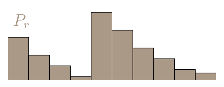
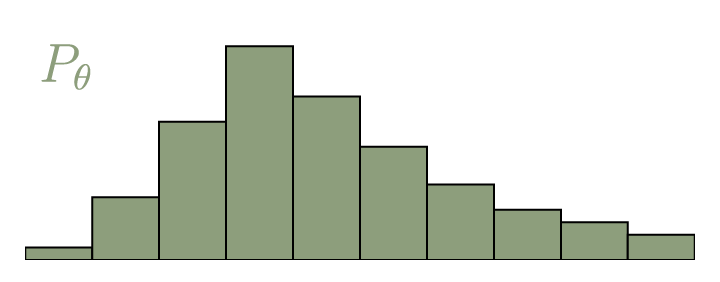
- Mathematical framework describing how to minimize the Earth Mover Distance, also called Wasserstein Distance $\mathrm{W}(P_r,P_{\theta}) = \inf_{\gamma \in \Pi} \, \sum\limits_{x,y} \Vert x - y \Vert \gamma (x,y)$
|
|
(Courtesy Vincent Herrmann)
Optimal Transport
- Mathematical framework describing how to minimize the Earth Mover Distance, also called Wasserstein Distance $\mathrm{W}(P_r,P_{\theta}) = \inf_{\gamma \in \Pi} \, \sum\limits_{x,y} \Vert x - y \Vert \gamma (x,y)$
- $\mathrm{W}(P_r,P_{\theta})=\inf_{\gamma \in \Pi} \, \langle \mathbf{D}, \mathbf{\Gamma} \rangle_\mathrm{F}$
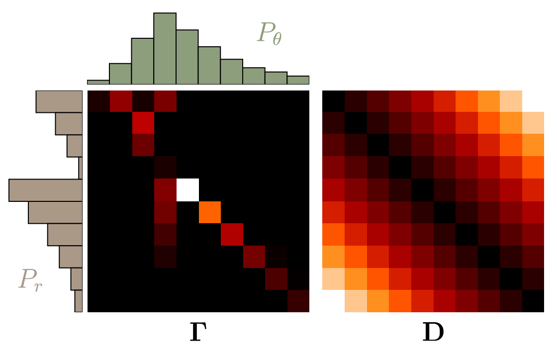
(Courtesy Vincent Herrmann)
Optimal Transport
Special case: empirical distribution (uniform distribution on every sample)
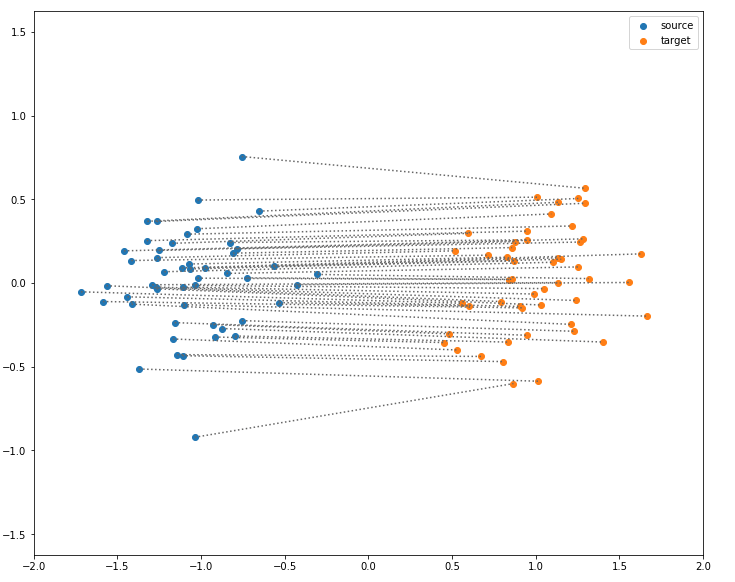
(Made with the optimal transport library POT)
$\mathrm{W}(P_r,P_{\theta}) = \inf_{\gamma \in \Pi} \, \sum\limits_{i,j} \Vert x_i - y_j \Vert \gamma (x_i,y_j)$ with $\gamma (x_i,y_j) \in \{0,1\}$
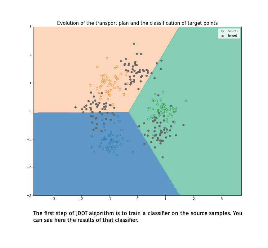
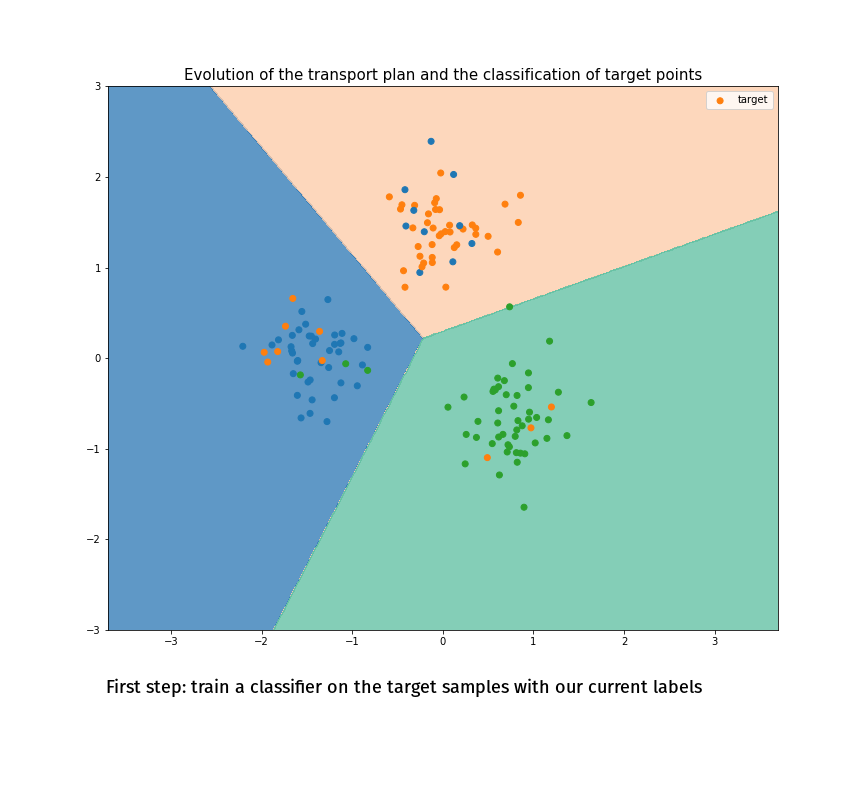
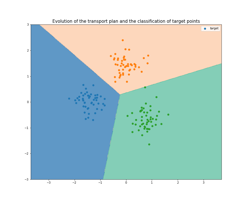
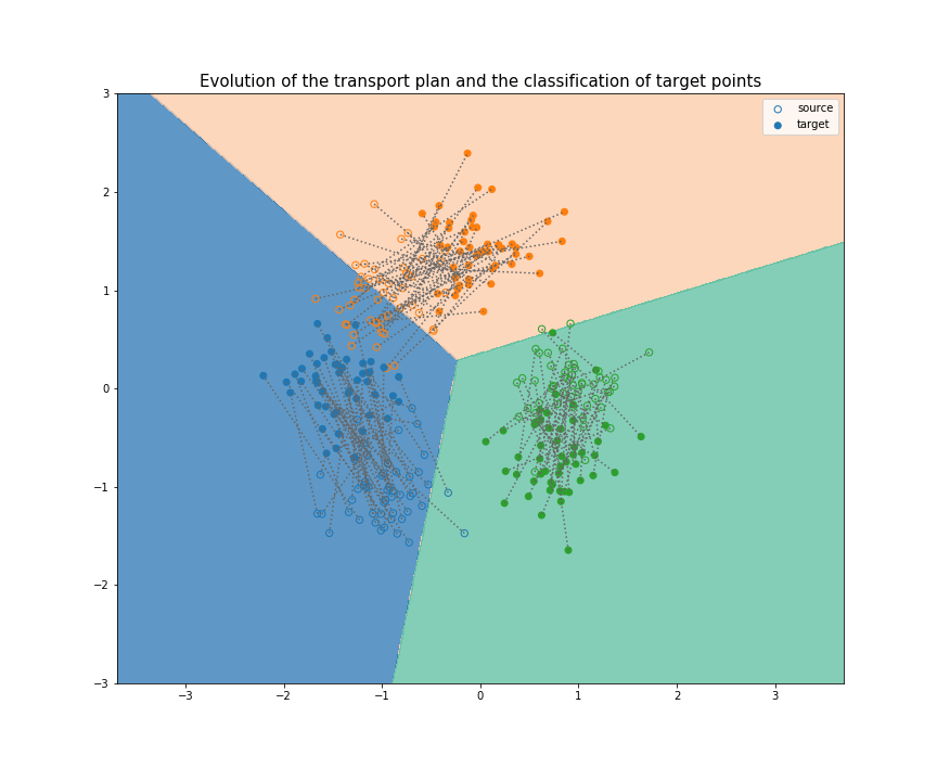
Joint Distribution Optimal Transportation
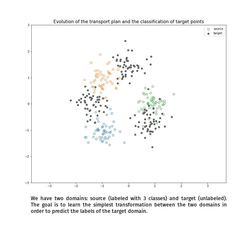
(Made with the optimal transport library POT)
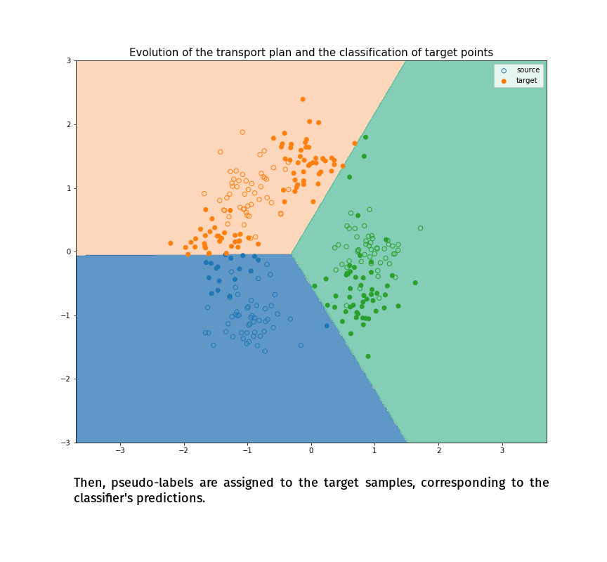
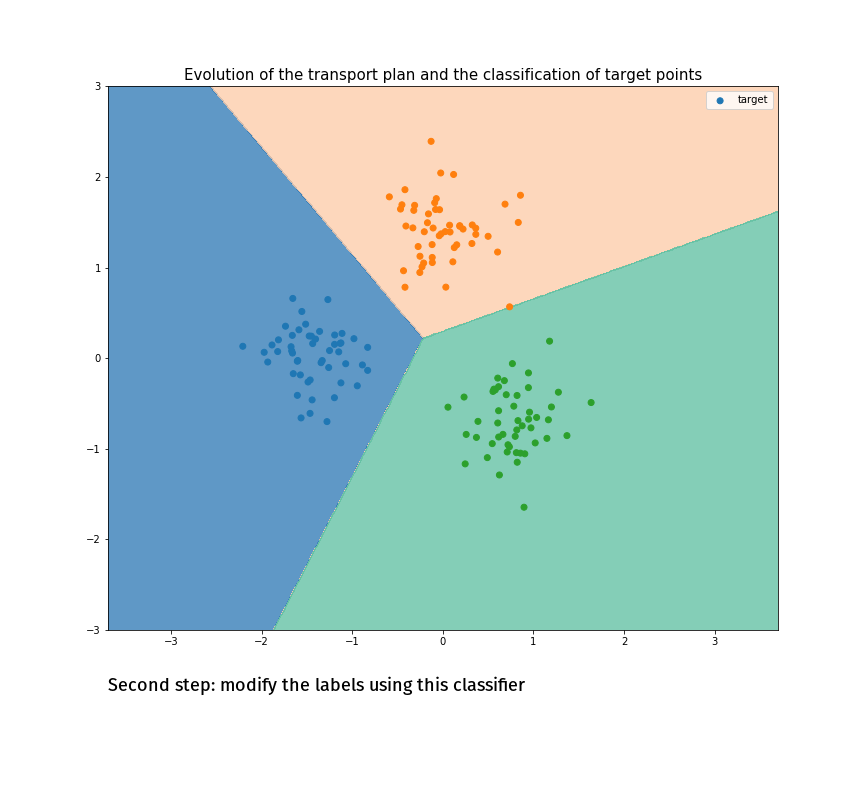
Joint Distribution Optimal Transportation
(Made with the optimal transport library POT)
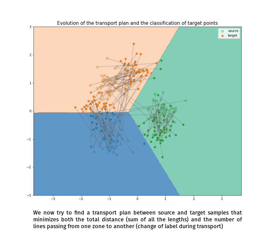
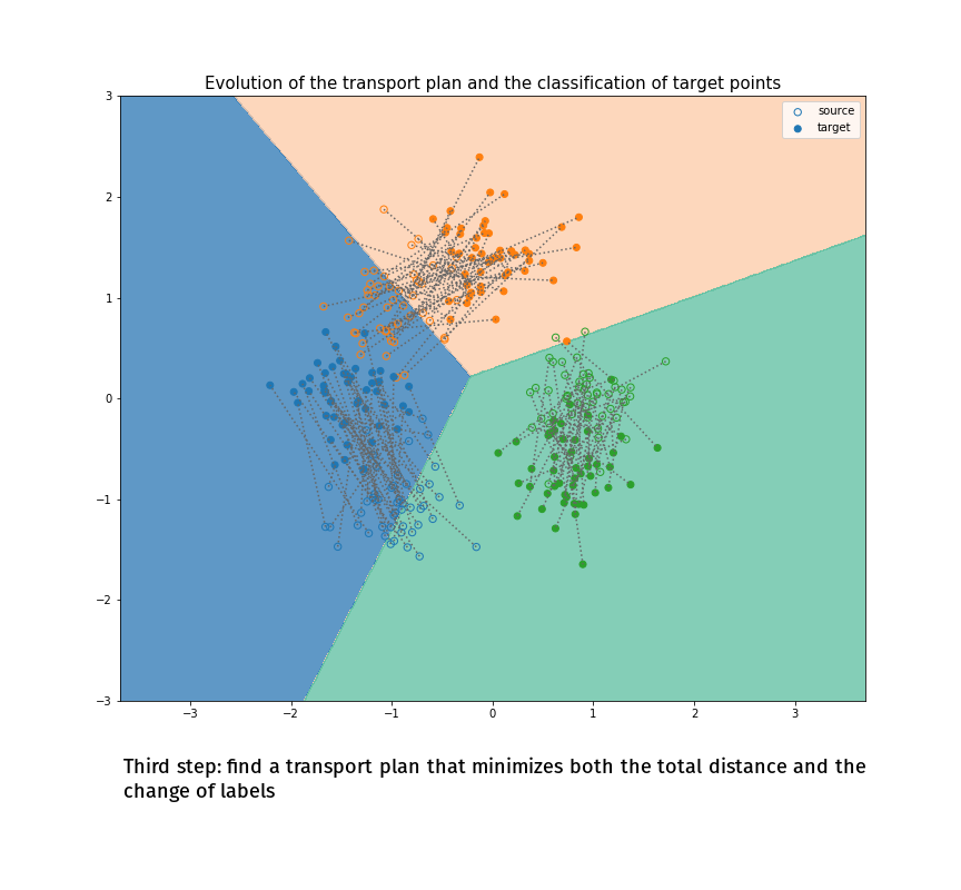
Joint Distribution Optimal Transportation
(Made with the optimal transport library POT)
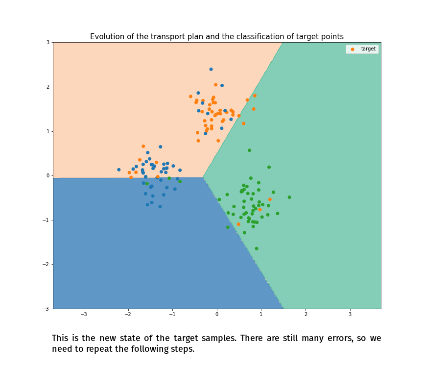
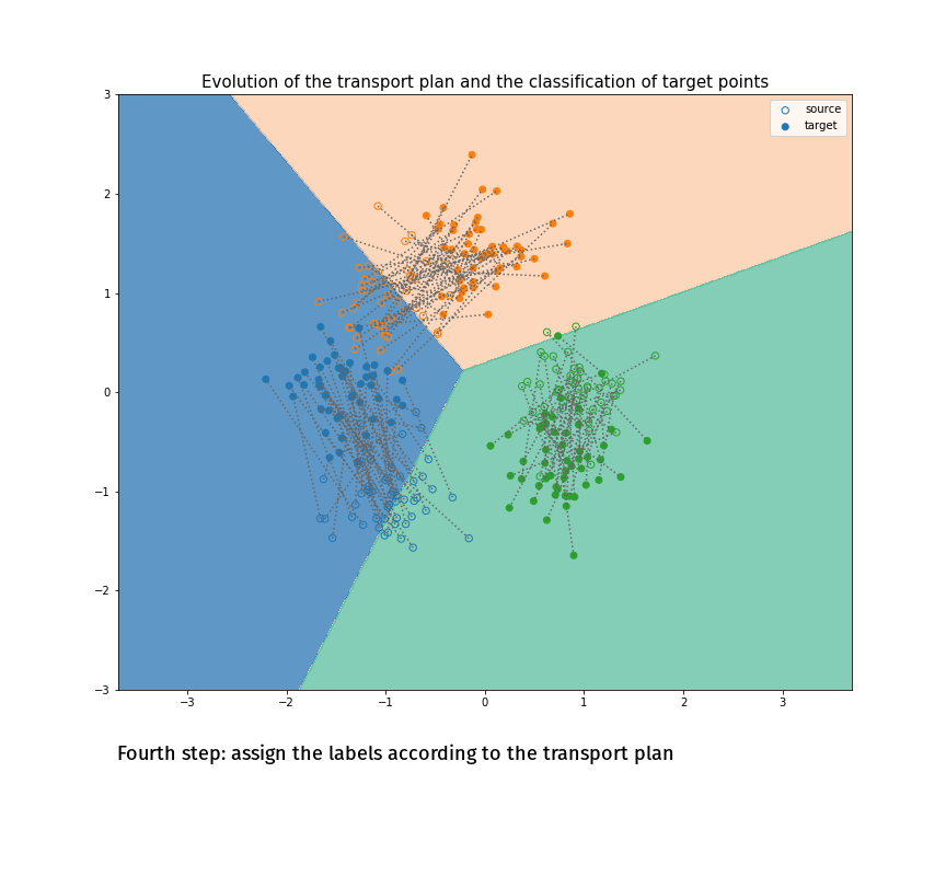
Joint Distribution Optimal Transportation
(Made with the optimal transport library POT)
Joint Distribution Optimal Transportation
(Courty et al., 2017)

(Made with the optimal transport library POT)
Joint Distribution Optimal Transportation
(Made with the optimal transport library POT)
Joint Distribution Optimal Transportation
(Made with the optimal transport library POT)
Joint Distribution Optimal Transportation
(Made with the optimal transport library POT)
Joint Distribution Optimal Transportation
(Made with the optimal transport library POT)
Joint Distribution Optimal Transportation
(Made with the optimal transport library POT)
Joint Distribution Optimal Transportation

(Made with the optimal transport library POT)
Joint Distribution Optimal Transportation
(Made with the optimal transport library POT)
Joint Distribution Optimal Transportation
(Made with the optimal transport library POT)
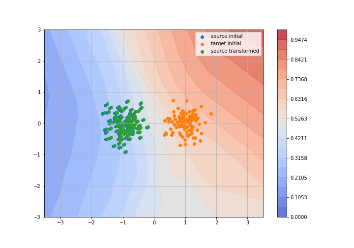
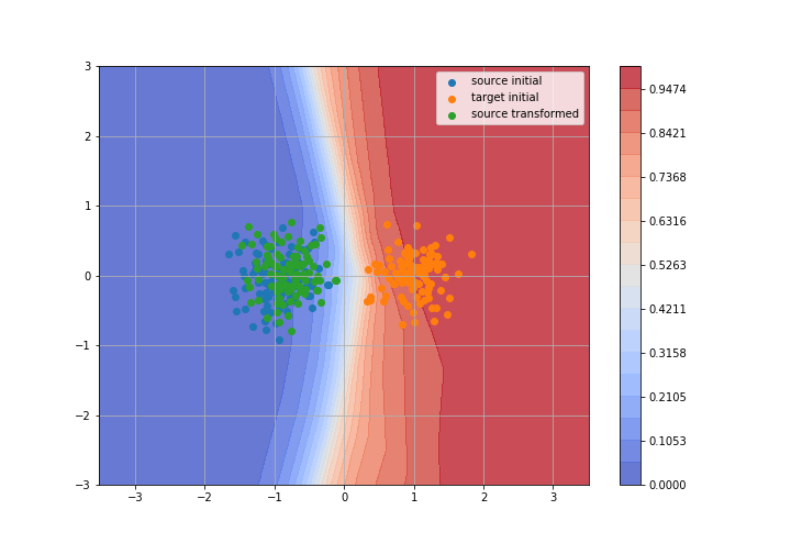
Adversarial Domain Adaptation
- Revolution in domain adaptation starting with Ganin et al., 2015
- Using GAN-like deep architectures to minimize the Jensen-Shannon divergence between our distributions
-
Adversarial domain adaptation framework:
- A conditional generator that takes a target input and tries to generate a source-like output
- A discriminator that tries to separate real source samples from source-like generated samples
- The generator tries to make the discriminator bad
- Almost all the recent DA papers are variations on that structure
Adversarial Domain Adaptation
Example of CycleGAN (Zhu et al., 2017)
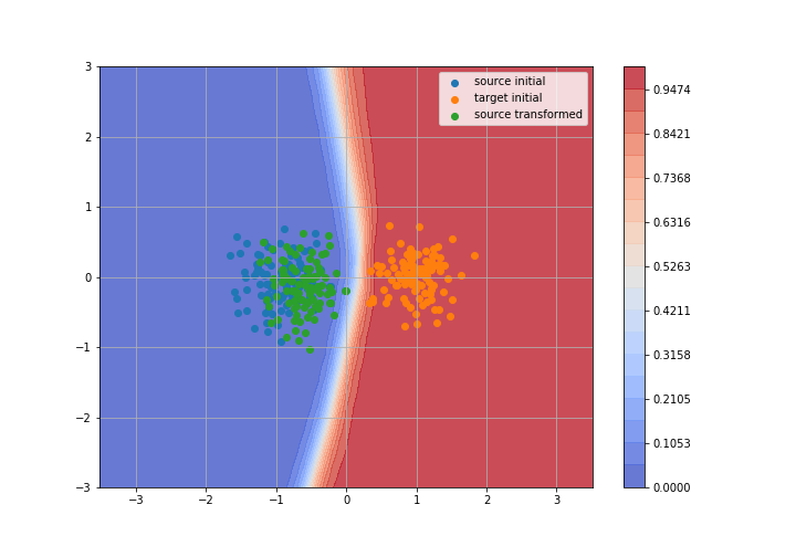
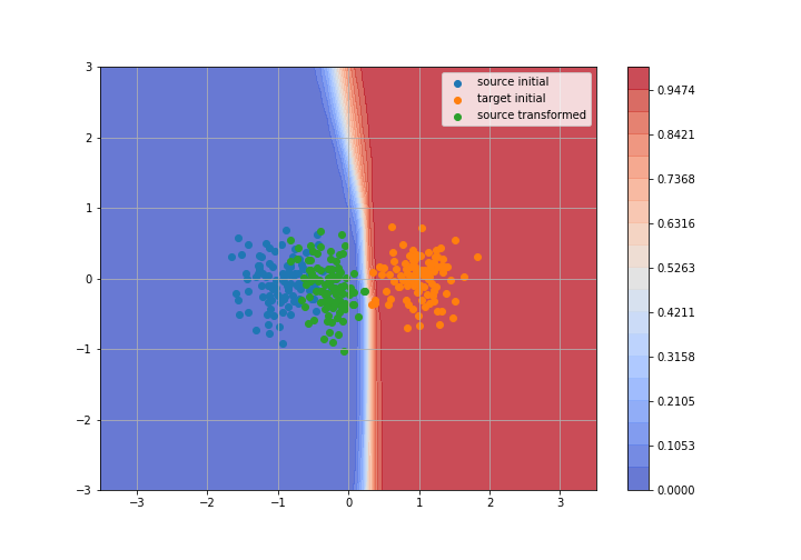
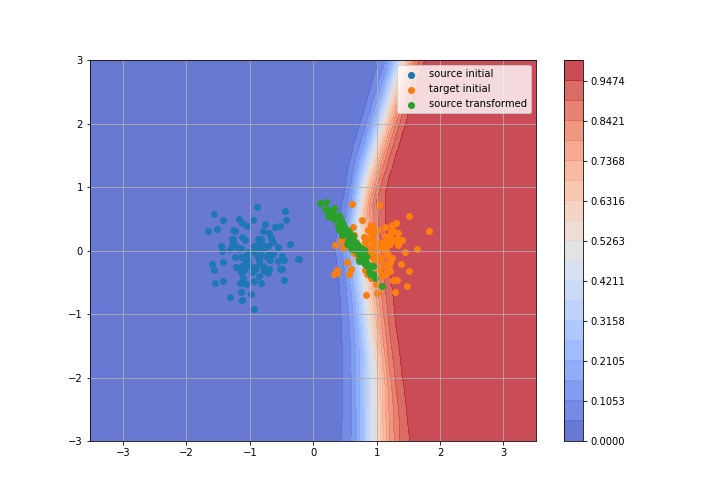
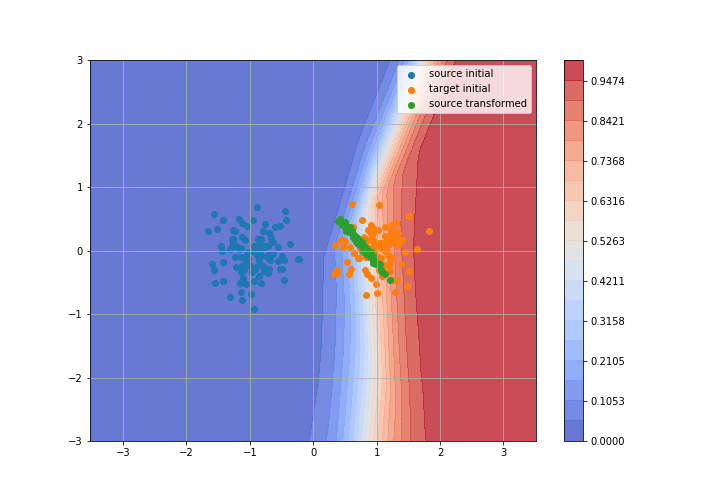
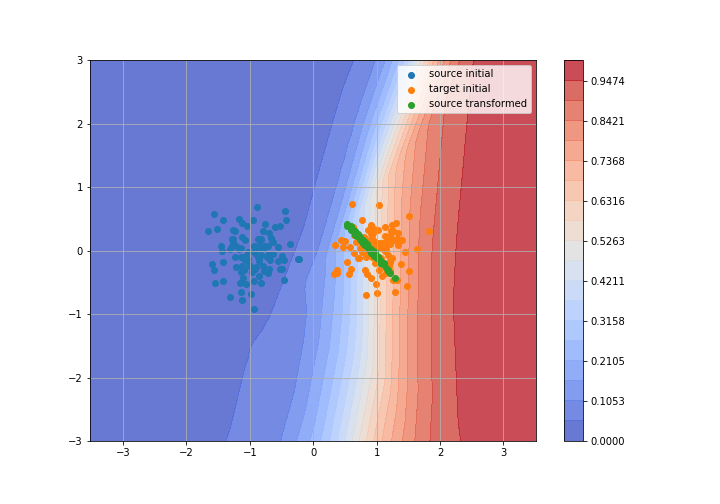
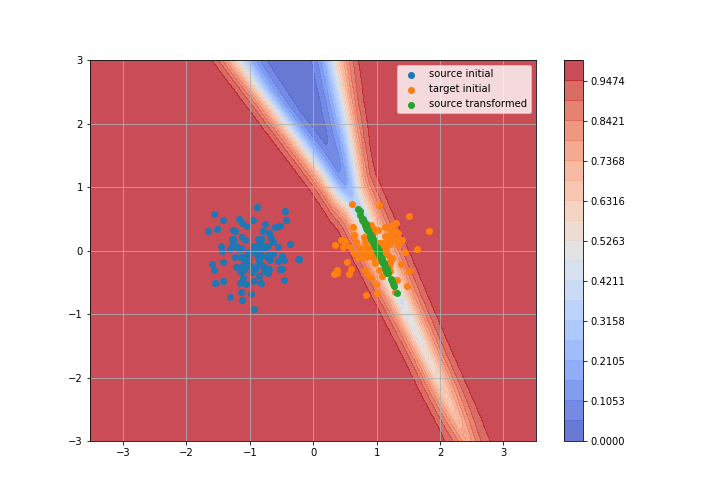
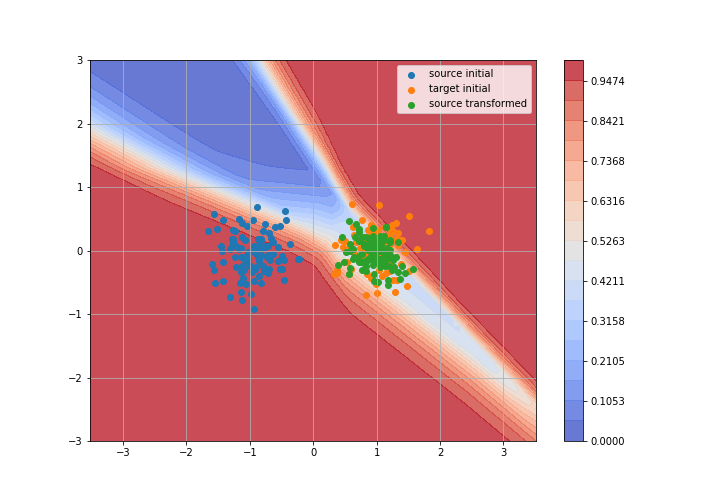
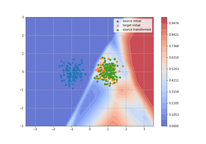
Adversarial Domain Adaptation
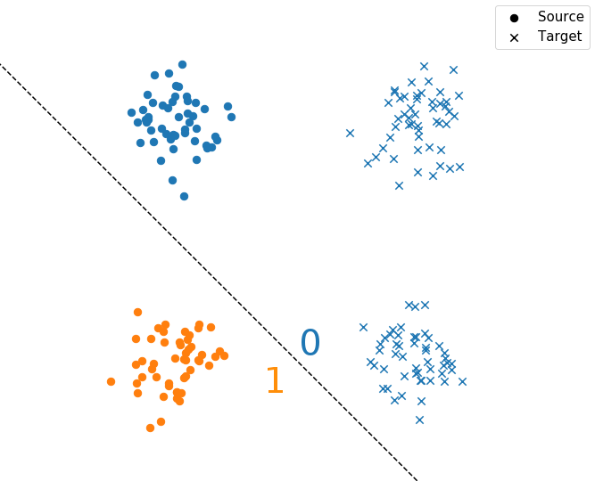
Toy example: 2D gaussians
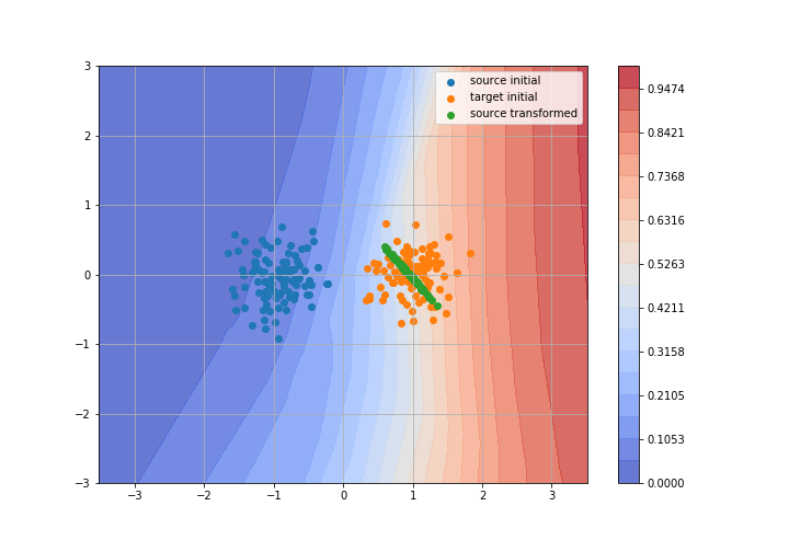
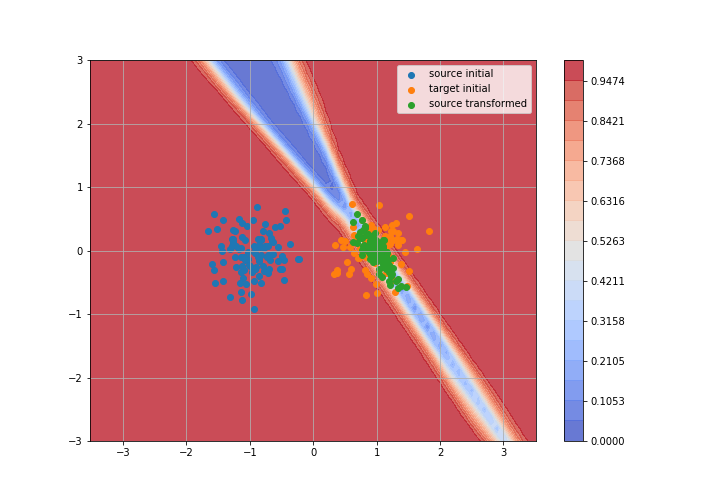
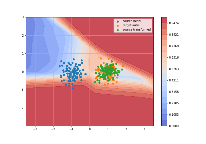
Adversarial Domain Adaptation
Toy example: 2D gaussians
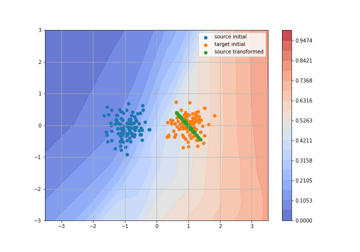
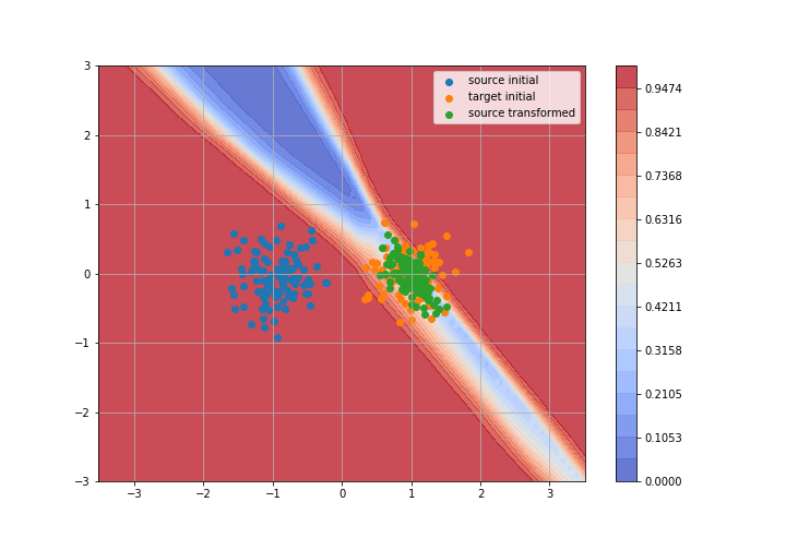
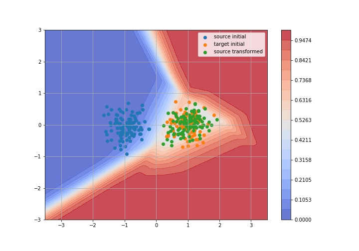
Adversarial Domain Adaptation
Toy example: 2D gaussians
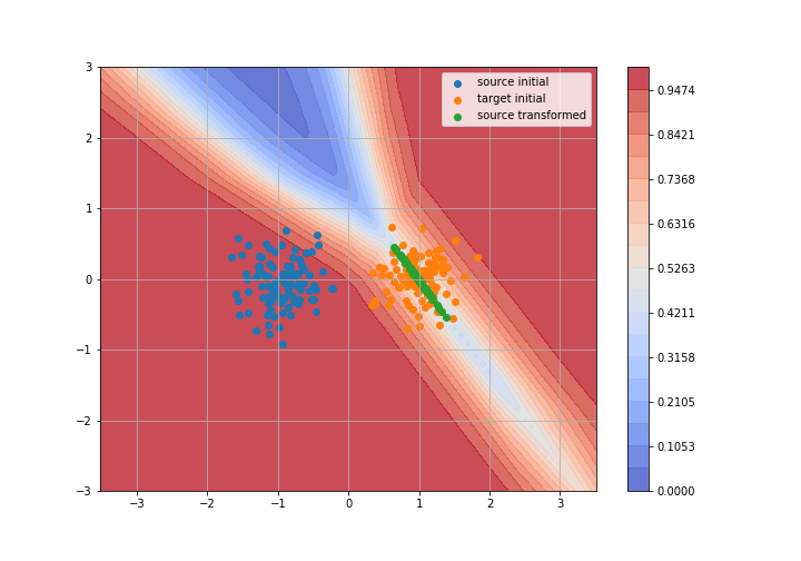
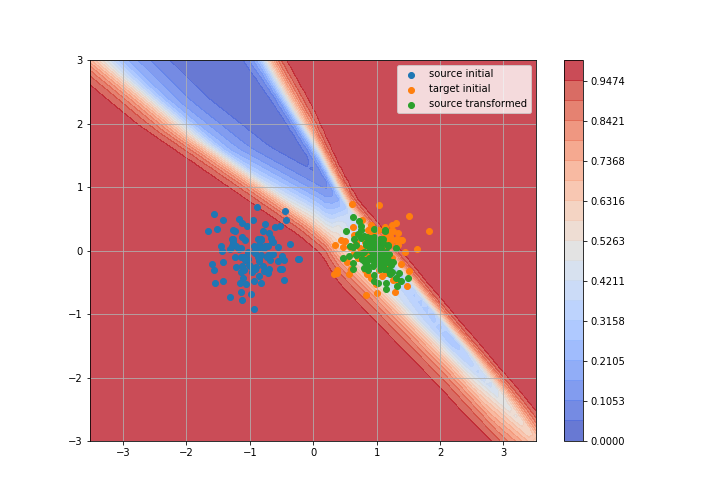
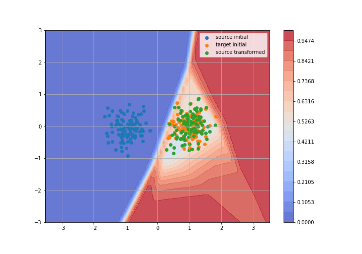
Adversarial Domain Adaptation
Toy example: 2D gaussians
Adversarial Domain Adaptation
Toy example: 2D gaussians

Adversarial Domain Adaptation
Toy example: 2D gaussians
Adversarial Domain Adaptation
Toy example: 2D gaussians
Adversarial Domain Adaptation
Toy example: 2D gaussians
Adversarial Domain Adaptation
Toy example: 2D gaussians
Adversarial Domain Adaptation
Toy example: 2D gaussians
Adversarial Domain Adaptation
Toy example: 2D gaussians
Adversarial Domain Adaptation
Toy example: 2D gaussians
Adversarial Domain Adaptation
Toy example: 2D gaussians

Adversarial Domain Adaptation
Toy example: 2D gaussians
Adversarial Domain Adaptation
Toy example: 2D gaussians
Adversarial Domain Adaptation
Toy example: 2D gaussians
Adversarial Domain Adaptation
Toy example: 2D gaussians
Adversarial Domain Adaptation
Toy example: 2D gaussians
Adversarial Domain Adaptation
Toy example: 2D gaussians
Adversarial Domain Adaptation
Toy example: 2D gaussians
Adversarial Domain Adaptation
Toy example: 2D gaussians
UNsupervised Image-to-Image Translation (UNIT)
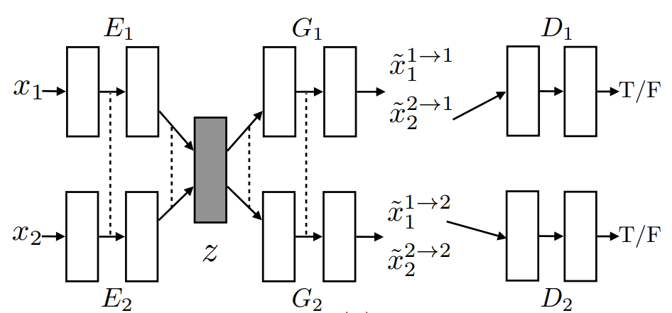
- Hypothesis: shared latent-space
- Training: VAE and GAN
UNsupervised Image-to-Image Translation (UNIT)
Results
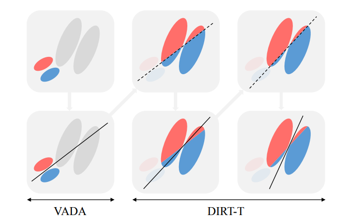
State-of-the art algorithm: VADA-DIRT-T
- Virtual Adversarial Domain Adaptation (VADA)
- Adversarial Method: find an embedding space invariant between the two domains and a hypothesis that classify the source in this embedding space
-
Cluster Assumption: the decision-boundary should not cross high-density regions
⇒ the output probability should be extreme (high-confidence)
⇒ $\min_{\theta} \mathbb{E}_{x \in \mathcal{D_t}}[-h_{\theta}(x) \log(h_{\theta}(x))] $

- Virtual Adversarial Training: the hypothesis should be invariant to slight perturbation of the input (adversarial examples). We can minimize the KL divergence between $h_{\theta}(x)$ and $h_{\theta}(x+r)$ for $||r||<\epsilon$
State-of-the art algorithm: VADA-DIRT-T
Evolution of domain adaptation results
On the MNIST-SVHN benchmark
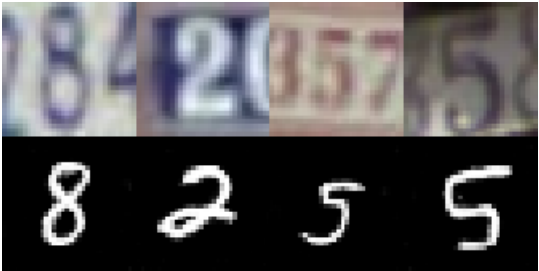
SVHN (source) → MNIST (target)
| Year | Algorithm | Accuracy |
|---|---|---|
| 2015 | SA | 59.3 |
| DANN | 73.8 | |
| 2016 | DRCN | 82.0 |
| DSN | 82.7 | |
| DTN | 90.7 | |
| 2017 | UNIT | 90.5 |
| GenToAdapt | 92.4 | |
| DA_assoc | 97.6 | |
| 2018 | DIRT-T | 99.4 |
Resources
- Awesome Transfer Learning: curated list of papers, datasets and other resources in domain adaptation and transfer learning (https://github.com/artix41/awesome-transfer-learning)
- Domain Adaptation in 2017: blog article (https://artix41.github.io/static/domain-adaptation-in-2017/)
- Introduction to optimal transport for GANs: blog article (https://vincentherrmann.github.io/blog/wasserstein/
- Computational Optimal Transport (2017): online book by Peyré and Cuturi, excellent visual introduction to OT